Time Series Forecast Algorithm-DSP

Introduction for DSP Algorithm

10 minute read

Time series forecasting refers to using historical time series data to predict future values. Time series data typically consists of time and corresponding values, such as resource usage, stock prices, or temperature. DSP (Digital Signal Processing) is a digital signal processing technique that can be used for analyzing and processing time series data.

Discrete Fourier Transform (DFT) is a commonly used algorithm in the field of DSP. DFT is a technique that transforms time domain signals into frequency domain signals. By decomposing time domain signals into different frequency components, the characteristics and structures of the signals can be better understood and analyzed. In time series forecasting, DFT can be used to analyze and predict the periodicity and trend of signals, thereby improving the accuracy of forecasts.

Crane uses commonly used techniques in the field of Digital Signal Processing (DSP), such as Discrete Fourier Transform (DFT) and autocorrelation function, to identify and predict periodic time series.

This article will introduce the implementation process and parameter settings of DSP algorithms to help readers understand the principles behind the algorithms and apply them to practical scenarios. (The related code is located in the pkg/prediction/dsp directory.)

Flow

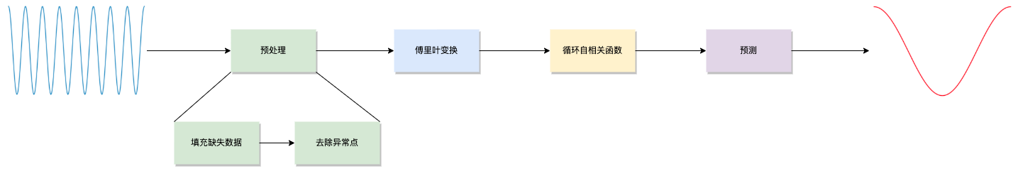
Preprocessing

Data imputation

It is common for monitoring data to be missing at certain time points, and Crane will fill in the missing sampling points based on the surrounding data. The method is as follows:

Assume that the sampling data between the m-th and n-th sampling points are missing (m+1<n). Let the sampling values at points m-th and n-th be $v_m$ and $v_n$. Then, let $$\Delta = {v_n - v_m \over n-m}$$, the missing data between m-th and n-th are $$v_m+\Delta , v_m+2\Delta , …$$

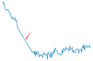
Remove outliers

Occasionally, there may be some extreme outlier data points in the monitoring data, and there are many reasons for these outliers, such as:

The monitoring system fills missing sampling points with 0 values;
The monitored component reports incorrect indicator data due to its own bugs;
The application consumes resources far beyond normal operation when starting up.

These extreme outlier points will interfere with the periodic judgment of the signal and need to be removed. try as follows:

Select the $P99.9$ and $P0.1$ of all sampling points in the actual sequence as the upper and lower threshold values, respectively. If a sampling value is lower than the lower limit or higher than the upper limit, set the value of the sampling point to the previous sampling value.

Discrete Fourier Transform

Performing a fast discrete Fourier transform (FFT) on the monitored time series (assuming a length of $N$) generates a spectrogram that intuitively displays the signal’s frequency spectrum as “impulses” at various discrete points $k$. The vertical height of each impulse represents the “amplitude” of the periodic component corresponding to $k$, where $k$ takes values in the range $(0,1,2, … N-1)$.

$k = 0$ corresponds to the “DC component” of the signal, which has no effect on the signal’s periodicity and can be ignored.

Due to the conjugate symmetry of the first half and second half of the frequency spectrum sequence after the discrete Fourier transform, the graph is symmetric about the axis and only the first half $N/2$ needs to be considered.

The period corresponding to $k$ is $$T = {N \over k} \bullet SampleInterval$$

To determine whether a signal has a period $T$, it is necessary to observe at least double of length $T$. Therefore, the maximum period that can be identified through a sequence of length $N$ is $N/2$. Thus, $k = 1$ can be ignored.

Therefore, the range of values for $k$ is $(2, 3, … , N/2)$, corresponding to periods of $N/2, N/3, …$ This is the “resolution” of period information that FFT can provide. If a signal’s period does not fall on $N/k$, it will be spread over the entire frequency domain, leading to “frequency leakage.”

Fortunately, in actual production environments, the applications we usually encounter (especially online services) have regular cycles, often on a “daily” basis. Certain businesses may exhibit a “weekend effect,” where behavior on weekends differs from that on weekdays. However, when observed at the “weekly” level, they still exhibit good periodicity.

Crane does not attempt to discover periodicity of arbitrary lengths, but instead specifies several fixed cycle lengths ($1d、7d$)for detection. The sequence length $N$ is ensured to be a multiple of the target detection period $T$ by trimming or padding the sequence, for example: $$T=1d，N=3d；T=7d，N=14d$$.

We have collected some monitoring indicators for applications from production environments and saved them in CSV format under the pkg/prediction/dsp/test_data directory.

For example, the input0.csv file contains 8 days of CPU monitoring data for an application, with the corresponding time series shown in the following graph:

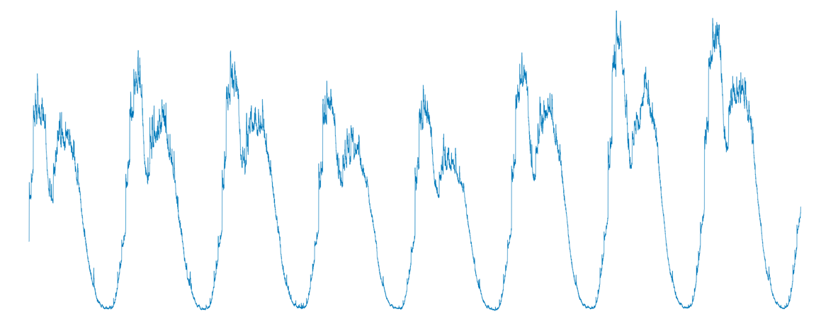
As we can see, although the data varies from day to day, the overall “pattern” is still quite consistent.

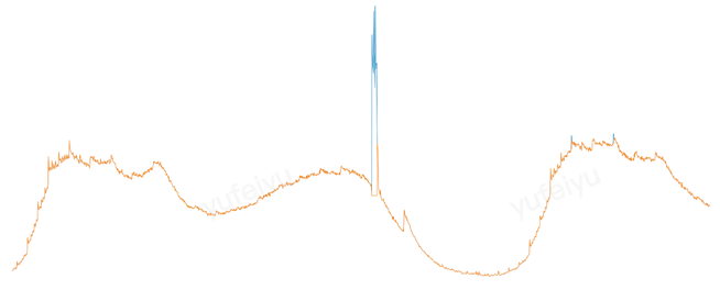
Performing an FFT on this sequence yields the following frequency spectrum:

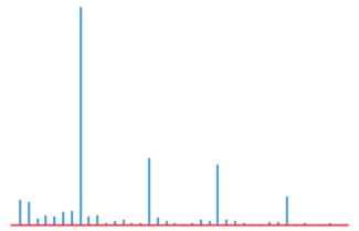
We can see that the “amplitude” is significantly higher at several points than at other points in the spectrum. These points can be used as our “candidate periods” for further verification.

The previous explanation was based on our intuitive judgement, how does Crane select its “candidate periods”?

Performing a random permutation of the original sequence $\vec x(n)$ results in the sequence $\vec x’(n)$. Applying the FFT to $\vec x’(n)$ yields $\vec X’(k)$, let $P_{max} = argmax|\vec X’(k)|$.
Repeat the above operation 100 times to obtain 100 values of $P_{max}$, then set $P_{threshold}$=$P99$.
Compute the FFT of the original sequence $\vec x(n)$ to obtain $\vec X(f)$. Traverse $k = 2, 3, …$, and if $P_k = |X(k)| > P_{threshold}$, then add $k$ to the list of candidate periods.

Auto Correlation Function

Auto Correlation Function (ACF) is the cross-correlation of a signal with itself at different time points. In simple terms, it is a function of the time lag between two observations that measures the similarity between them.

Crane uses circular autocorrelation function (Circular ACF), which first extends the time series of length $N$ by using $N$ as the period. This means that the sequence $\vec x(n)$ is copied over the interval $…, [-N, -1], [N, 2N-1], …$, resulting in a new sequence $\vec x’(n)$ that is used for analysis.

The correlation coefficient between $\vec x’(n+k)$ and $\vec x’(n)$ is computed for each shift $k=1,2,3,…N/2$, where $\vec x’(n)$ is shifted by $k$. $$r_k={\displaystyle\sum_{i=-k}^{N-k-1} (x_i-\mu)(x_{i+k}-\mu) \over \displaystyle\sum_{i=0}^{N-1} (x_i-\mu)^2}\ \ \ \mu: mean$$

Instead of directly computing the ACF using the definition mentioned above, Crane uses the following formula and performs two FFT operations to calculate the ACF in $O(nlogn)$ time. $$\vec r = IFFT(|FFT({\vec x - \mu \over \sigma})|^2)\ \ \ \mu: mean,\ \sigma: standard\ deviation$$

The ACF is represented graphically as shown below, where the x-axis represents the time lag $k$ and the y-axis represents the autocorrelation coefficient $r_k$, which reflects the degree of similarity between the shifted signal and the original signal.

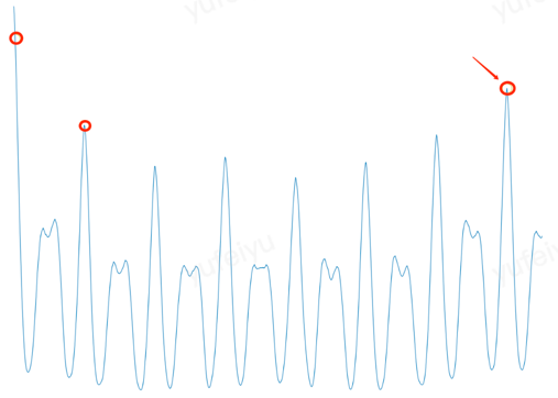
Crane verifies if the autocorrelation coefficient at each candidate period is located at the “peak of the curve”. It selects the candidate period that corresponds to the highest peak as the primary cycle (fundamental period) of the entire time series and uses it for prediction.

How to determine the “peak of the curve”?

Crane selects a section of the curve on each side and performs linear regression separately. If the slope of the left and right lines after regression are greater than and less than zero respectively, then the point is considered to be at a “peak”.

Predict

Based on the primary cycle obtained in the previous step, Crane provides two methods to fit (predict) the time series data for the next cycle.

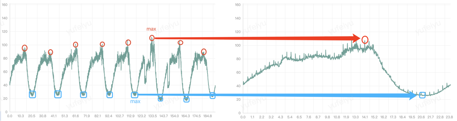
maxValue

The first method is to select the maximum value at time $t$(e.g. 6:00 PM) for each of the past few cycles, and use it as the predicted value for the next cycle at time $t$.

fft

The second method is to perform FFT on the original time series to obtain a frequency spectrum sequence, remove the “high-frequency noise”, and then perform IFFT (inverse fast Fourier transform). The resulting time series is used as the predicted result for the next cycle.

Applicate

Crane provides TimeSeriesPrediction as a CRD, allowing users to predict various time series data, such as CPU utilization rates of the workload, application QPS, and so on.

apiVersion: prediction.crane.io/v1alpha1
kind: TimeSeriesPrediction
metadata:
  name: tsp-workload-dsp
  namespace: default
spec:
  targetRef:
    apiVersion: apps/v1
    kind: Deployment
    name: test
    namespace: default
  predictionWindowSeconds: 7200 # Provide the predicted data for the next 7200 seconds (2 hours) and write it to the status field in Crane
  predictionMetrics:
    - resourceIdentifier: workload-cpu
      type: ExpressionQuery
      expressionQuery:
        expression: 'sum (irate (container_cpu_usage_seconds_total{container!="",image!="",container!="POD",pod=~"^test-.*$"}[1m]))' # Query statement to retrieve historical monitoring data
      algorithm:
        algorithmType: "dsp" # Specify the prediction algorithm as dsp
        dsp:
          sampleInterval: "60s" # The sampling interval for monitoring data is 1 minute.
          historyLength: "15d"  # Pull the monitoring metrics from the past 15 days as the basis for prediction
          estimators:           # Specify the prediction method, including maxValue and fft. Multiple estimators with different configurations can be specified for each method, and Crane will select the one with the highest fitting degree to generate the prediction results. If not specified, fft will be used by default
            fft:
              - marginFraction: "0.2"
                lowAmplitudeThreshold: "1.0"
                highFrequencyThreshold: "0.05"
                minNumOfSpectrumItems: 10
                maxNumOfSpectrumItems: 20

The meanings of some dsp parameters in the example above are as follows:

maxValue

marginFraction: After fitting the next cycle of the sequence, each predicted value is multiplied by 1 + marginFraction. For example, if marginFraction = 0.1, it means multiplying by 1.1. The purpose of marginFraction is to magnify or reduce the predicted data by a certain proportion.

fft

lowAmplitudeThreshold: The lower limit of spectral amplitude. All frequency components below this lower limit will be filtered out.

highFrequencyThreshold: The upper limit of frequency. All frequency components above this upper limit will be filtered out. The unit is Hz. For example, if you want to ignore the cycle component with a length less than 1 hour, set highFrequencyThreshold = 1/3600.

minNumOfSpectrumItems: The minimum number of frequency components to be retained.

maxNumOfSpectrumItems：The maximum number of frequency components to be retained.

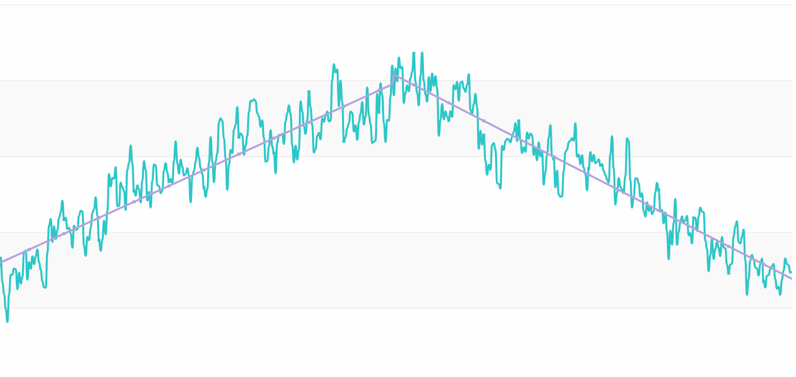
In simple terms, the fewer frequency components retained, the lower the upper frequency limit, and the higher the spectral amplitude lower limit, the smoother the predicted curve will be, but some details will be lost. Conversely, more detailed features are preserved with more frequency components retained, resulting in a more jagged curve.

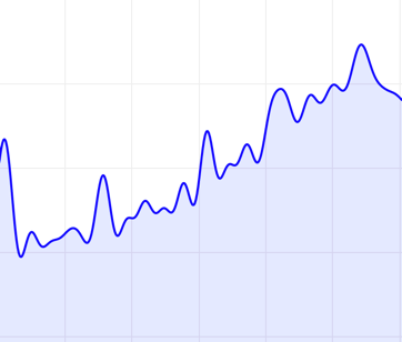
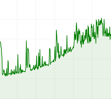
Below are two predicted curves for the same time period. The blue and green lines have different highFrequencyThreshold values of $0.01$ and $0.001$, respectively. The blue curve filters out more high frequency components, resulting in a smoother curve.

There is no single parameter configuration that is suitable for all time series. Usually, it is necessary to adjust the algorithm parameters according to the characteristics of the application indicators in order to obtain the best prediction results. Crane provides a web interface that allows users to intuitively see the prediction results after adjusting the parameters. The steps are as follows:

Modify the parameters of estimators in TimeSeriesPrediction.
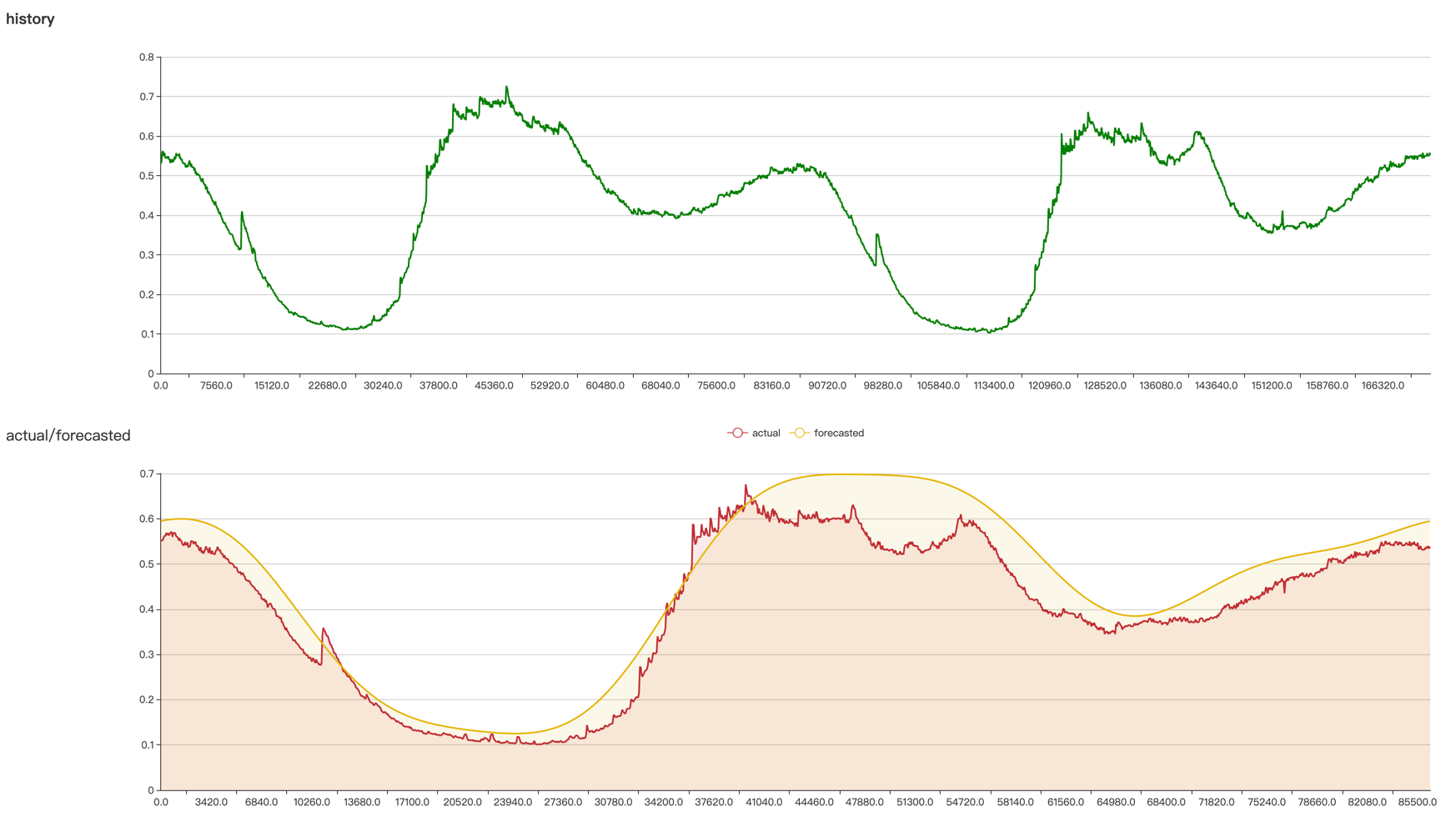
Access the api/prediction/debug/<namespace>/<timeseries prediction name> of the Crane HTTP server to view the parameter effect (as shown below).

The above steps can be executed multiple times until satisfactory prediction results are obtained.

Debug locally through port-forward.

The port of the Crane HTTP server is set by the –server-bind-port startup parameter of Crane, and the default value is 8082.

Open the terminal

$kubectl -n crane-system port-forward service/craned 8082:8082
Forwarding from 127.0.0.1:8082 -> 8082
Forwarding from [::1]:8082 -> 8082

Open the browser and visithttp://localhost:8082/api/prediction/debug/<namespace>/<timeseries prediction name>